
A Simple Guide to Gradient Boosting of Decision Trees in SAP IBP

In this series, I will break down the available forecasting algorithms in IBP to make them easier to understand and implement in your demand planning processes. Among the most complex models that IBP offers is Gradient Boosting of Decision Trees (hereafter simply referred to as “Gradient Boosting”). Gradient Boosting is classified as an “ensemble machine learning algorithm,” which means it combines many simple models into one ensemble to achieve better forecasting results. The idea works like this:
We build an initial model to the data and see how well it forecasts (how well it predicts future results).
Then, we build a second model, focusing on accurately predicting the cases where the first model performed poorly.
The combination of the above two models is expected to be better than just using the initial, single model.
Repeat this model generation many times based on the shortcomings of the last model in the series. Each new model created is a step in the direction of minimizing prediction errors, hence the name “gradient boosting.”
The “decision trees” part of the name describes the modeling approach used by the algorithm. The purpose of a decision tree is to determine which observations (independent variables) affect the outcome, and what point in the process, and in what way, do the variables affect those results.
For example, say you are a movie theater who is trying to figure out how many tickets will be sold. There are many factors that affect ticket sales, such as day of the week, ticket prices, and whether there’s a new movie out. You’ve been collecting data about how many tickets were sold every day, as well as data about all these other factors (you made a note when ticket prices fluctuated or when a new hit movie came out). You input all those variables and all ticket sales into a tree-building model.
The model looked at all these variables, and it determined that whether or not a hit movie comes out is a big factor in ticket sales, so this becomes a split in the tree. It also determined that day of the week is a big factor in ticket sales, and it determined whether hit-movie-coming-out should be factored before or after price of a ticket. Once the algorithm determines all of the splits, it can then use the tree to determine future ticket sales.

In the above example, price is one of the most determinate factors for how will tickets will sell. If the price is less than $20, then the day of the week is the next most important factor, and then other variables are considered. But if price is more than $20, then whether a movie that will entice viewers to flock to theaters becomes a more prominent factor, or predictor variable, in determining ticket sales.
Once the model has made many trees and calculated the errors and shortcomings of each tree, the final step the algorithm takes is assigning a weight to each tree. The final prediction is the weighted sum of all the trees.
Gradient Boosting of Decision Trees has various pros and cons. One pro is the ability to handle multiple potential predictor variables. There are other algorithms, even within IBP, that can handle multiple predictor variables; however, Gradient Boosting can outshine other algorithms when the predictor variables have multiple dependencies between them, rather than being standalone independent variables with no impact on the other variables in the model.
Gradient boosting also has cons, the most impactful of which is its tendency to overfit. Overfitting means that a model matches too closely to the historical data. At first glance, it may seem like a great thing if the model perfectly matches the past data, but the risk with overfitting is the model is biased to the sample (the test data set provided to the model) rather than properly estimating for the entire population (the entire data set). The tree model is also very reliant on the sample test data, so if the data set is not truly representative of the entire population, Gradient Boosting will be unable to make good predictions. Additionally, Gradient Boosting of Decision Trees requires a *lot* of computing, making it system-intensive and increasing the time it takes to run forecasts.
With these pros and cons in mind, if Gradient Boosting is right for your dataset, you’ll need to know how to configure it in IBP.
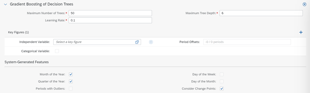
Pictured above are the default values IBP suggests for a Gradient Boosting model. Let’s go through each input:
Maximum Number of Trees: This field is used to specify the maximum number of times the model should try to create a successive tree to lessen the shortcomings (residual errors) of the previous tree. Choosing a large maximum number of trees will mean that the model is more prone to overfitting. Many potential trees also require more computations and runtime, so it’s not recommended to have a large number for longer time series (more than 250 data points).
Maximum Tree Depth: The maximum number of levels in a tree. The algorithm builds many trees, so the trees don’t need to be very deep. Usually, smaller trees are preferred, with between 4 and 8 levels.
Learning Rate: When all the trees are created and the model is adding up the final results, the learning rate determines the weights applied to the trees. The lower the learning rate, the less the contribution of each tree to the model as you keep adding trees. If you decrease the learning rate, you should increase the maximum number of trees to prevent overfitting. If you work with short time series, you can apply very shallow trees (1, 2, or 3 levels), a small learning rate (0.001-0.01), and a larger number of trees (for example, 1000).
If I were starting from scratch, I would start with the default inputs that IBP provides. Then, change an input and run the model again to see how the error changes. Continue changing inputs and rerunning the model and compare the various inputs to the various error measures to determine the inputs that produce the best results, keeping mind that you want to prevent overfitting.
Independent Variable: These are all the variables you keep track of which might affect your sales. Factors like holidays, pricing data, promotions, etc.
Categorical Variable: Categorical Variables are events that occurred in the past and are expected to occur again in the future. Using categorical variables, you can mark different events using codes like 100, 200, etc in separate key figures intended to store these variables. In this way, if 100 represents a promotion, and Gradient Boosting recognizes that seeing the value “100” in a key figure tends to increase sales by 20%, then Gradient Boosting will forecast higher in future periods in which you input “100.”
Period Offsets: Say Valentine’s Day affects your sales- but it’s not just February 14, it’s the days leading up to February 14th as well which have higher sales numbers. Period offsets allow you to clone and temporarily shift values of independent variables to offset periods so the model can better calculate a forecast for those periods.
System-Generated Features: Are your sales greater in February than in March? Are they greater in Q4 than in Q2? Do your products sell better on Saturday than on Tuesday? If you check these boxes, Gradient Boosting will use calendar data to identify various potential types of seasonality, if it exists as a factor in your dataset’s results.
Periods with Outliers: This can be used alongside the Pre-Processing Step Outlier Correction with No Correction. Checking this box will allow the model to recognize (but not correct) outliers, so that the outliers do not affect future forecasting results.
Change Points: This can be used alongside Forecast Automation. Change points occur when something fundamentally changes in a dataset, such as the trend slope changes, or the average of the historical data shifts. The system can recognize change points and will expect the average level of values to continue unchanged, following the most recent change point.
Now that we understand Gradient Boosting in its entirety, here’s how I’d summarize:
Gradient Boosting of Decision Trees is a model that recognizes that various independent variables can have various effects on the final sales results. It takes all those variables and figures out which ones affect the results, in what way they affect the results, at what point they affect the results. All of those “decision points” make a branch based on whether that condition is TRUE or FALSE, and each of those branches will have more branches off them, ending in leaves, which are the results.
So Gradient Boosting will make a tree, then try to figure out the shortcomings of that tree, and make another tree, all while keeping those shortcomings in mind. This process is repeated with each successive tree, and in the end, you have a bunch of trees, each one trying to be marginally better than the last. And Gradient Boosting will look at all those trees, assign weights to them, and use them all to produce the final results on whatever dataset you’re running the model on. You can choose the maximum number of trees it tries to make, how deep each tree goes, and how much the model weighs each successive tree.